BGS LS10 — Joint SMF + wp(rp) + ΔΣ
This page documents the joint summary-statistic run on the nine DESI BGS VLIM stellar-mass-threshold (Mstar) samples from the Legacy Survey DR10 (LS10) footprint. For each sample the script computes stellar mass function (SMF), projected correlation function wp(rp), and excess surface density ΔΣ(rp), together with a full 100-region spatial jackknife covariance matrix.
Scripts
scripts/measure_bgs_joint_smf_wp_ds_hsc_des.py— SMF + wp + ΔΣ(HSC) + ΔΣ(DES)scripts/measure_bgs_joint_hsc.py— SMF + wp + ΔΣ(HSC)scripts/measure_bgs_joint_smf_ds_des.py— SMF + ΔΣ(DES)scripts/measure_bgs_ds_hsc.py— stand-alone ΔΣ(HSC)scripts/measure_bgs_joint_ds_multisurvey.py— ΔΣ(DES + HSC + KiDS)scripts/plot_joint_measurements.py— per-sample figure with ratio and correlation panels
Configuration
rp bins   : 40 log-spaced bins in [10^{-2.5}, 10^{1.5}] Mpc  (0.003–31.6 Mpc)
SMF bins  : 0.1 dex steps from mstar_min to 12.5
pi_max    : 100 Mpc
n_jk      : 100 spatial regions (K-means on (RA, Dec))
cosmo     : Planck18 flat ΛCDM  (H0=67.4, Ω_m=0.315)
source cat: HSC Y3 and/or DES Y3 (precomputed lens–source pair sums)
Weighting
Note
Two weight variants are computed for each sample via --weight-variant all:
uniform — all weights = 1 (no imaging systematic correction). Output filename: e.g.
joint_smf_wprp_deltasigma_hsc_des.h5.sys-comb — WEIGHT_COMB from the MCMC combined systematic model at NSIDE 64, as recommended by the
sys_mappingdocumentation. Output filename: e.g.joint_smf_wprp_deltasigma_hsc_des-sys-comb.h5.
The weight file for each sample is
sys_mapping/data/sys_weights/{sample_id}_NSIDE0064_WEIGHTS.fits
with column WEIGHT_COMB = 1 / max(1 + Σ b̂ᵢ tᵢ(p), 0.01).
The weight filename and method are stored as HDF5 attributes in every
output group (weight_file, weight_nside, weight_method).
Run metadata
Sample ID |
log M★ min |
z min |
z max |
Area [deg²] |
Ngal |
|---|---|---|---|---|---|
LS10_VLIM_ANY_9.0_Mstar_12.0_0.05_z_0.08_N_0523486 |
9.00 |
0.05 |
0.08 |
18887 |
523 486 |
LS10_VLIM_ANY_9.5_Mstar_12.0_0.05_z_0.12_N_1432502 |
9.50 |
0.05 |
0.12 |
18950 |
1 432 502 |
LS10_VLIM_ANY_10.0_Mstar_12.0_0.05_z_0.18_N_2759238 |
10.00 |
0.05 |
0.18 |
18974 |
2 759 238 |
LS10_VLIM_ANY_10.25_Mstar_12.0_0.05_z_0.22_N_3308841 |
10.25 |
0.05 |
0.22 |
18978 |
3 308 841 |
LS10_VLIM_ANY_10.5_Mstar_12.0_0.05_z_0.26_N_3263228 |
10.50 |
0.05 |
0.26 |
18978 |
3 263 228 |
LS10_VLIM_ANY_10.75_Mstar_12.0_0.05_z_0.31_N_2802710 |
10.75 |
0.05 |
0.31 |
18974 |
2 802 710 |
LS10_VLIM_ANY_11.0_Mstar_12.0_0.05_z_0.35_N_1619838 |
11.00 |
0.05 |
0.35 |
18955 |
1 619 838 |
LS10_VLIM_ANY_11.25_Mstar_12.0_0.05_z_0.35_N_0541855 |
11.25 |
0.05 |
0.35 |
18889 |
541 855 |
LS10_VLIM_ANY_11.5_Mstar_12.0_0.05_z_0.35_N_0120882 |
11.50 |
0.05 |
0.35 |
18703 |
120 882 |
Summary figures
Stellar mass function (SMF)
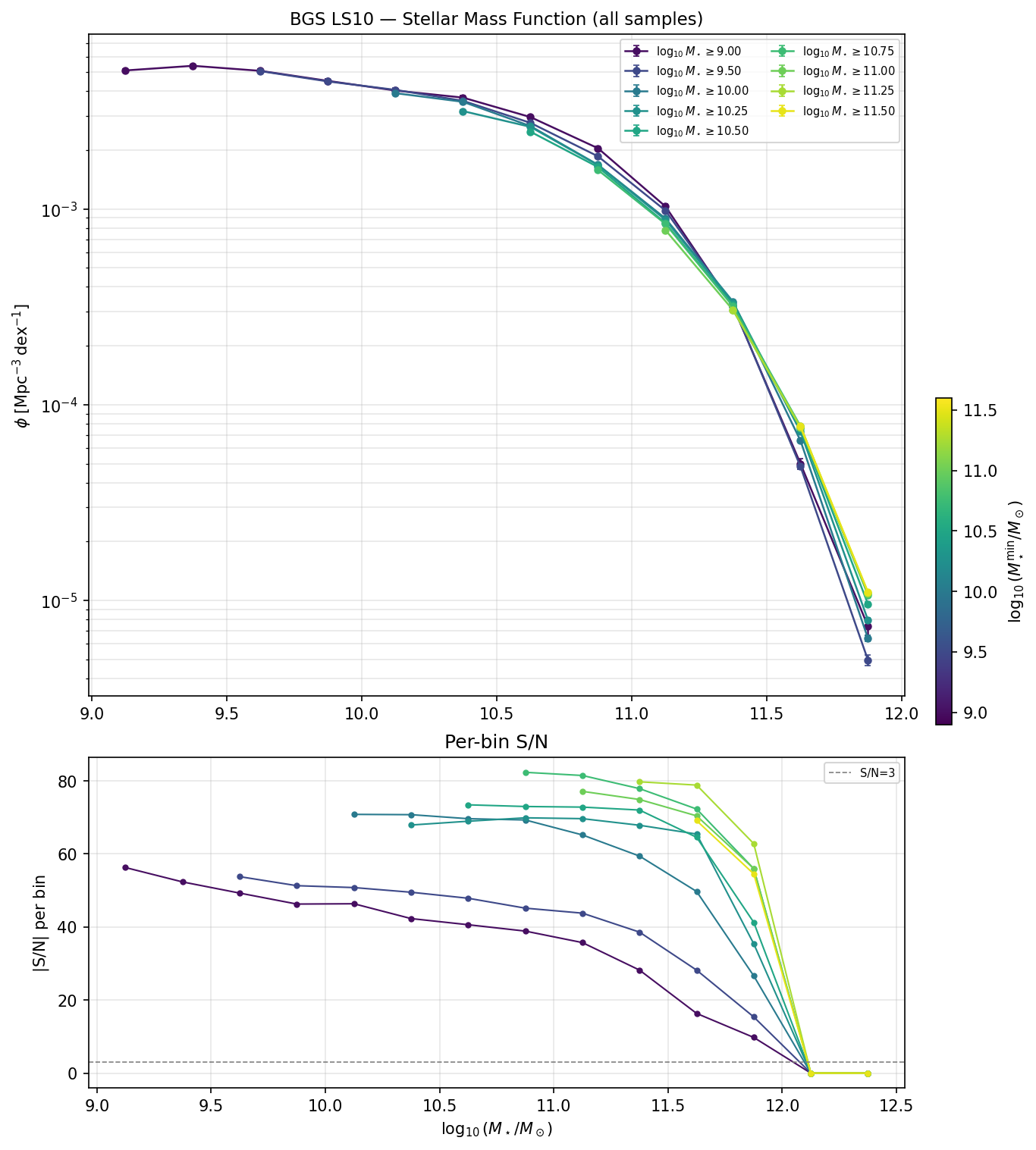
Top: SMF measurements with jackknife error bars for all 9 samples, colour-coded by log10(M★/M☉) threshold (viridis). Bottom: per-bin S/N = |φ| / σJK.
Projected correlation function wp(rp)
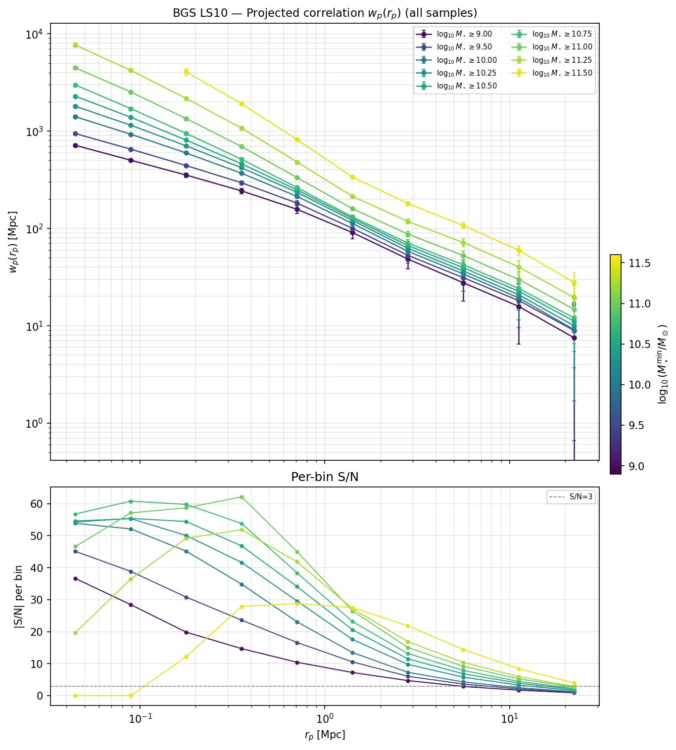
Top: wp(rp) measurements in Mpc (physical) for all 9 samples. Bottom: per-bin S/N.
Excess surface density ΔΣ(rp)
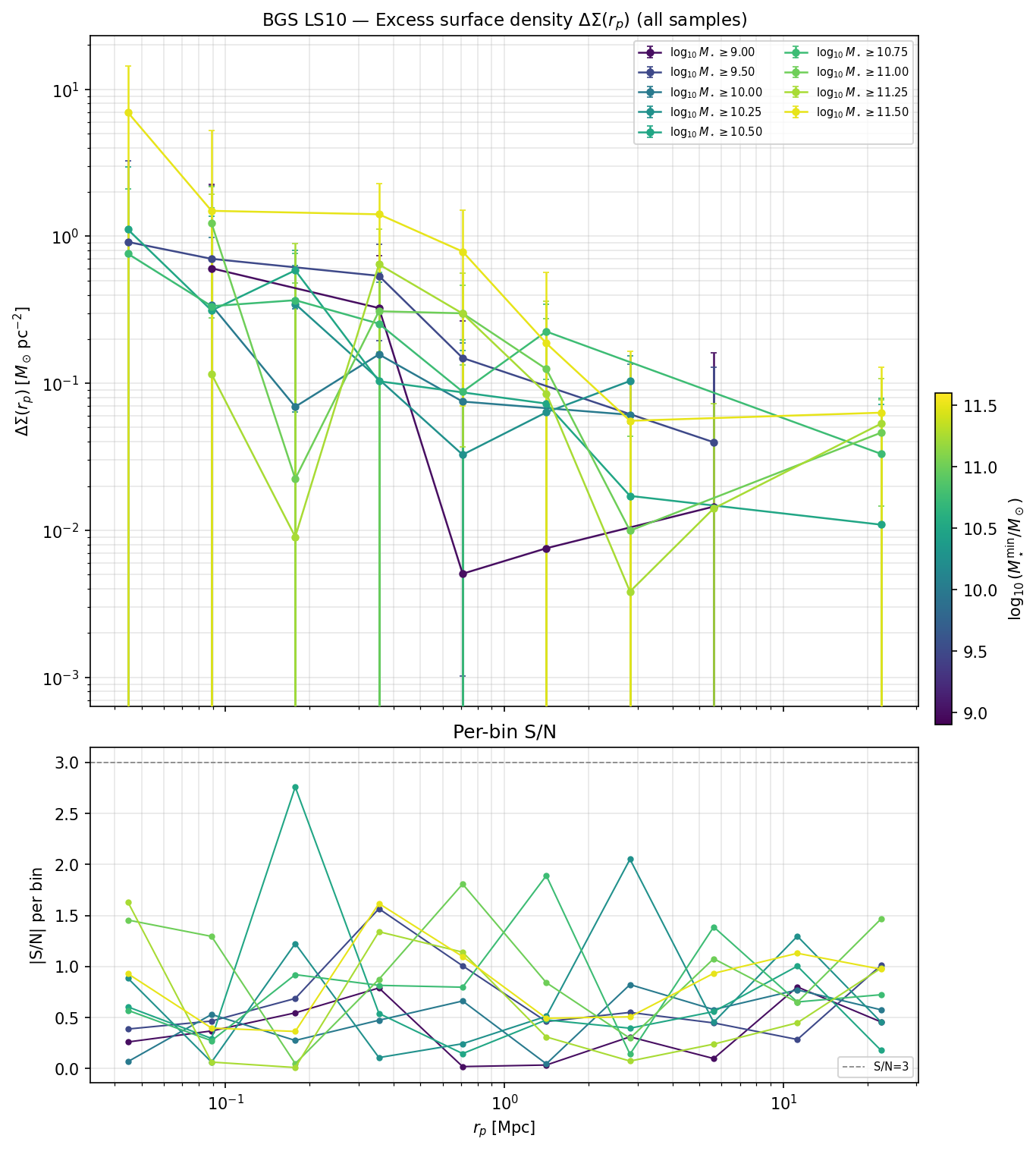
Top: ΔΣ measurements in M☉ pc-2 for all 9 samples. Bottom: per-bin S/N. Note the low S/N: low-redshift BGS samples barely overlap the HSC Y3 footprint, and the inner bins are dominated by noise.
Signal-to-noise summary
Total S/N = √(Σ (vali / erri)²) over all finite bins per statistic.
Sample |
SMF |
wp |
ΔΣ |
Joint |
|---|---|---|---|---|
|
141.4 |
54.3 |
1.4 |
151.5 |
|
139.0 |
74.1 |
2.5 |
157.5 |
|
175.0 |
98.3 |
1.7 |
200.7 |
|
171.0 |
107.7 |
3.0 |
202.1 |
|
164.5 |
113.8 |
3.2 |
200.1 |
|
166.9 |
125.1 |
3.0 |
208.6 |
|
140.2 |
125.8 |
3.5 |
188.4 |
|
128.5 |
98.7 |
2.7 |
162.1 |
|
88.0 |
57.3 |
2.9 |
105.1 |
Key observations:
SMF is extremely well measured across all samples (S/N ≈ 88–175 total). The jackknife captures both shot noise and large-scale sample variance.
w:sub:`p` is highly significant (S/N ≈ 54–126) and improves with increasing galaxy number density at intermediate mass thresholds (10.25–10.75).
ΔΣ is marginally detected (S/N ≈ 1.4–3.5 total). The low signal arises because the BGS VLIM samples live at low redshift (z ≲ 0.35) and only a small fraction of the survey area overlaps with the HSC Y3 footprint. ΔΣ bins at small rp are dominated by shape-noise. The ΔΣ information is still included in the joint data vector and covariance for completeness; future runs using a wider lensing source catalogue will improve this.
Technical notes
wp normalization with systematic weights
Note
When galaxy weights (wsys) are used, Corrfunc DDrppi_mocks
with weight_type="pair_product" returns weighted pair sums
Σi,j wi wj, not raw pair counts.
The convert_rp_pi_counts_to_wp normalization factors must therefore be
the sum of weights Σi wi, not the number of
galaxies N. For uniform weights Σw = N so the two are equivalent, but
for WEIGHT_COMB (mean ~ 1.02, std ~ 0.04) the difference is ~2 % in
amplitude. This fix is implemented in sum_stat/twopcf/projected.py.
Recommended model from gga_model
The BGS VLIM samples are stellar mass threshold cuts. The optimal model family depends on which observables are used as constraints.
Model class |
Predicts SMF? |
Notes |
|---|---|---|
|
No |
Zheng+2007 vanilla HOD (5 params). Does not predict the SMF, so SMF bins cannot constrain the model directly without abundance matching. |
|
No |
Threshold HOD with lensing constraint built in; useful for wp+ΔΣ alone. |
|
Yes |
Integrated CSMF (Guo+2018). Predicts φ, wp, ΔΣ self-consistently from the conditional stellar mass function P(M★ | Mhalo). Recommended for the full joint vector. |
|
Yes |
Updated ICSMF (Guo+2019). Minor parametrisation differences from Guo18; use as a cross-check. |
Recommendation: use Guo18ICSMFModel (or Guo19ICSMFModel) for
the full joint SMF + wp + ΔΣ fit. The ICSMF naturally connects
the stellar mass function and clustering statistics via the conditional
stellar mass function, so all three observables can be predicted
self-consistently from a single set of parameters without requiring
an external abundance-matching step.
ZuMandelbaum15HODModel is a good cross-check when fitting only
wp + ΔΣ and treating the SMF as a prior rather than a
constraint.
HODModel alone should be avoided: it predicts only wp (and
optionally ΔΣ via halo lensing), but not the SMF, so the 88–175 S/N SMF
data vector cannot be used as a constraint without layering an
abundance-matching model on top.